EcoGEM Lab
Build a food web. Change one relationship. Watch the consequences move through an ecosystem.
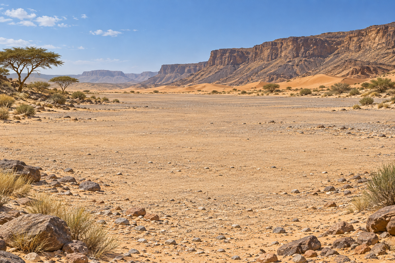
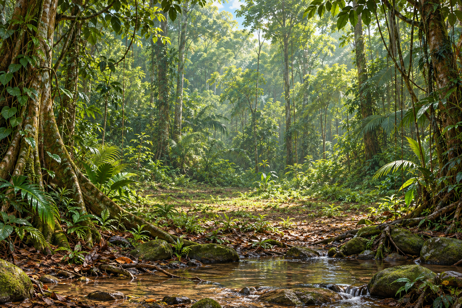
I’m a Grade 6 teacher in Ontario. I built this compact, illustrated lab to help students explain how a change travels through an ecosystem, then test and revise that explanation. Explore the Atlantic Ocean, Sahara Desert, and Amazon Rainforest with the food web, habitat, and graph together on one screen.
Open EcoGEM Lab ↗Teaching Grade 6? Start with the teacher guide →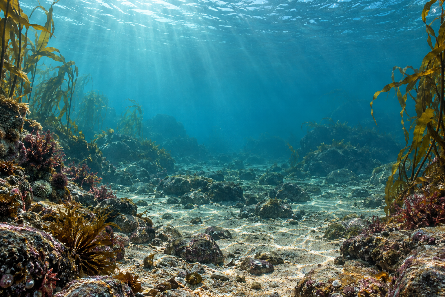
Why I built it
The original Ecology Lab was the experimental space at the centre of EcoGEM, my learning design built around Generate–Evaluate–Modify. Students could change a food web, test a prediction, and use what they observed to revise their explanation.
After Annenberg Learner closed, its original links stopped working. I found that the lab’s developer, Ginger Booth, still hosts a working HTML5 version. That surviving version is worth exploring in its own right. EcoGEM Lab is my independent adaptation of the experience, with three illustrated ecosystems. The standalone tool is a single screen; the EcoGEM learning experience embeds it with inquiry questions below.
Three places to investigate
Start with a place, then a question you can test. Each ecosystem offers a different set of selected feeding relationships. The Atlantic example begins with plankton. The Sahara example follows grasses and saltbush into insects, rodents, and predators. The Amazon example connects tree food resources, mammals, and birds of prey.
Click any organism to include or remove it, or to edit its selected feeding relationships. Change resource availability, run the model, and inspect the graph. Keep one run as a comparison, inspect exact values in the data table, or download the data for a closer look.
The three ecosystems save separately in your browser. There is no sign-up, and the lab sends no experiment data to a server.
How the model works
EcoGEM Lab is a simplified teaching model. Its purpose is to make direct and indirect effects visible, not to forecast populations in the Atlantic, Sahara, or Amazon. The model’s time steps and abundance units are illustrative. Real species vary by location, season, life stage, and many influences that are absent here.
Producers grow toward a resource limit. Consumers feed on their selected prey, gain a fraction of the food they consume, and lose abundance through mortality and crowding. Feeding saturates as food becomes plentiful. The resource slider changes the producer carrying capacity; its rainfall and nutrient labels are conceptual, not measurements.
Plant abundance represents available food such as leaves, fruit, seeds, and plankton. It does not mean that a tree dies each time an animal eats a leaf. The habitat uses layered depth, gentle movement, and shadows on a single canvas. Motion can be switched off and respects reduced-motion preferences. Positions and movement are illustrative, not simulated animal behaviour. Portraits are not to scale; their number rises with the square root of abundance, capped at 12 per group. Use the graph for exact values.
Equations and reproducibility
Producer growth is rᵢNᵢ(1 − (Nᵢ + 0.35ΣNother producers) / (K × resource)), before consumption. Consumers request prey at aᵢNᵢNⱼ / (hᵢ + ΣNselected prey). Shared requests cannot exceed the prey available in that substep. Consumer growth is eᵢ × food consumed − mᵢNᵢ − cᵢNᵢ².
The engine uses 20 simultaneous substeps per model step. Abundance below 0.1 is treated as extinction, and an extinct species returns only when deliberately reintroduced. Runs stop at step 1,000. The same setup and changes produce the same result; the model contains no random events.
Changing a web pauses the simulation and records the intervention. Reset starts the current web again with its default abundances. A new preset starts a fresh web. A kept comparison is preserved. CSV contains every step’s abundances; the experiment JSON also contains the initial state, settings, intervention states, comparison, and model version.
Parameter values are educational choices, not measurements fitted to these organisms. The original Ecology Lab’s numerical model was not recovered. This adaptation uses newly written code and will not reproduce historical worksheet values.
From trying the tool to teaching with it
Begin with a short orientation so students can use the three views. Then move through competition, connected food webs, and disturbance. Each investigation follows Generate–Evaluate–Modify: make a prediction, compare it with evidence, and revise the explanation.
This sequence supports Ontario’s Grade 6 Science and Technology curriculum, especially B2.5 (ecological interrelationships) and A1.2/A1.5 (investigation and communication). It offers discussion of biodiversity and resilience, with a separate Ontario invasive-species extension. It does not cover the entire biodiversity strand. Read the official curriculum ↗
Open the full EcoGEM experience for the embedded lab and student notebook. The teacher guide includes lesson openings, exact experiment setups, discussion prompts, assessment, access supports, and curriculum connections. Download the guide as a PDF.
Feeding-relationship sources
The feeding relationships in each ecosystem draw on the following research and species accounts.
Atlantic Ocean
- NOAA: Copepods—Cows of the Sea ↗
- Schmidt (2010), Food and feeding in Northern krill ↗
- Suca et al. (2018), Feeding dynamics of Northwest Atlantic small pelagic fishes ↗
- Bowman et al. (2000), Food of northwest Atlantic fishes and two common species of squid ↗
- Trophic Ecology of Atlantic Cod off Cape Cod, 2001–2004 ↗
- Smithsonian National Zoo: Gray seal ↗
- COSEWIC (2011), Atlantic bluefin tuna assessment ↗
Sahara Desert
- FAO: Desert locust frequently asked questions ↗
- Feedipedia: Desert grass (Panicum turgidum) ↗
- Osborn & Helmy (1980), The contemporary land mammals of Egypt (including Sinai) ↗
- Degen (1988), Ash and electrolyte intakes of the fat sand rat consuming saltbush ↗
- Daly & Daly (1973), On the feeding ecology of Psammomys obesus ↗
- Brahmi et al. (2012), First quantitative data on the diet of the fennec fox in Algeria ↗
- León (2020), Cerastes cerastes—MoroccoHerps ↗
- Cole & Wilson (2015), Felis margarita (Carnivora: Felidae) ↗
- IUCN/SSC Cat Specialist Group: Sand cat ↗
Amazon Rainforest
- New York Botanical Garden: Bertholletia excelsa taxon account ↗
- Julliot & Sabatier (1993), Diet of the red howler monkey in French Guiana ↗
- Wisconsin National Primate Research Center: Red howler monkey ↗
- Aquino & Bodmer (2004), Plantas útiles en la alimentación de primates en la cuenca del río Samiria, Amazonia Peruana ↗
- The demography of a resource specialist in the tropics: Cecropia trees and the fitness of three-toed sloths (2019) ↗
- Sloths like it hot: ambient temperature modulates food intake in the brown-throated sloth (2015) ↗
- Aguiar-Silva et al. (2014), Food habits of the harpy eagle, a top predator from the Amazonian rainforest canopy ↗
- Emmons (1987), Comparative feeding ecology of felids in a neotropical rainforest ↗
Original work and credits
EcoGEM Lab author: Andrew Morris. Grade 6 teacher in Ontario; learning design, independent simulation, and website experience. Habitat and organism illustrations were created with ImageGen for this project.
The original Ecology Lab was developed by Ginger Booth with the Harvard-Smithsonian Science Media Group for Annenberg Media’s The Habitable Planet. Booth dates the original to 2006 and the HTML5 revision to 2015. The new simulator and teacher guide use newly written code and text, an independently specified numerical model, and new illustrations. They do not bundle the original lab’s code, artwork, or lesson text. The historical EcoGEM design paper is a separate document and includes screenshots of the original experience.
The course-wide Interactive Labs credits also name Ian Albinson, Kurt House, Eric Klopfer, Eli Meir, Jaimie Miller, and Alison Plante alongside Booth. Those are credits for the course’s collection of labs, not a claim that every contributor worked on Ecology specifically.
What is inspired, and what is new?
The linked food-web, habitat, and population-graph approach, and the ability to change a web and watch its consequences, are acknowledged inspirations. The three ecosystem selections, feeding-relationship research, illustrations, interface implementation, equations, and accompanying teaching guide were developed for this project. EcoGEM Lab is independently developed for the EcoGEM learning sequence. It is not an official sequel or an authorized release by the original authors.
APA reference for the original simulation
Booth, G. (2015). Ecology Lab [HTML5 simulation]. The Habitable Planet. https://gingerbooth.com/html5/interactives/ecology/ecology.html (Original work published 2006)
In-text acknowledgement: (Booth, 2006/2015).
Further background
- Ginger Booth’s portfolio: development and revision dates
- The Habitable Planet development partnership
- Course appendix: Interactive Labs credits on printed page 185 (legacy document; availability may vary)
- Annenberg Learner’s closure notice
- Andrew Morris’s EcoGEM learning design
This is an independent adaptation and is not endorsed by Annenberg Learner or the original authors.